Tutorial #4: Classifying the SEDs of Herbig Ae/Be stars
Last modification: D. Baines January 2013
The overall goal of this tutorial is to classify the Spectral Energy Distribution (SED) of a number of Herbig Ae/Be stars (young intermediate mass stars).
Background: The SEDs of Herbig Ae/Be stars fall roughly into two groups: Group I sources have a relatively strong far-IR flux, which is energetically comparable with the flux in the near-IR showing an almost flat spectral energy distribution. Group II sources show a similar near-IR excess as group I sources but their flux falls off strongly towards the far-IR. These were first classified by Meeus et al (2001, A&A, 365, 476), see below figure.
Dullemond and Dominik (2004, A&A, 417, 159) provided a physical explanation for this difference: Group II sources have an outer disk which is protected against direct stellar radiation by a puffed-up inner disc. If the outer disc emerges from the inner disc's shadow, i.e. has a large flaring angle, then its SED resembles that of a Group I source.
Tutorial:
Open TOPCAT (for a large memory, open the topcat jar file using the following command: java -Xmx2048m -jar topcat.jar ).
Download the The et al (1994) Herbig Ae/Be catalogue by doing the following:
VO -> Vizier Catalogue Service
Click 'All Rows', select Output Columns as 'standard', select 'By Keyword' and type 'Herbig Ae/Be' in the Keywords box. Click 'Search Catalogues'
Select J/A+AS/104/315 - Member of Herbig Ae/Be stellar group (The et al 1994), Output Columns equals standard, and press OK.
8 tables are now downloaded into TOPCAT. To check what each of these tables are open View -> Table Parameters, and check the Description.
We want the second table: J.A+AS.104.315-2, which is Table 1 of The et.al. (1994) and contains the Herbig Ae/Be members and candidate members (108 rows by 9 columns).
Gathering IRAS and 2MASS photometry for each source:
Select Multiple cone search (VO-> Multicone).
In the Keywords field type 'IRAS Point' and click 'Submit Query'
Select the IRAS Point Source Catalogue, version 2 (II/125), the input table as J_A+AS_104_315_table1, RA column as _RAJ2000, DEC column as _DEJ2000, the search radius column as 10 arcsec, the Output Mode as 'New joined table with best matches', and Error Handling as 'ignore'.
The result is a table that contains 64 rows (i.e. 64 cross matches with the IRAS PSC were found), and contains the 9 columns from the The et. al. catalogue, 16 columns from the IRAS PSC and a column, called _r, which gives the cross match angular distance or separation in degrees.
Create a subset of this cross matched table by selecting Views -> row subsets and in the Row Subsets window select Subsets ->New subset. Choose a subset name and select the best matches, column _r, by typing '$10 < 0.001' into the Expression field.
This produces a subset of 29 sources. In the main TOPCAT window chose this subset by selecting the Row Subset field.
Select again the VO -> Multicone and this time type '2MASS' in the Keywords field and click 'Submit Query'.
Select the 2MASS PSC catalogue (II/246), the input table as the new 29 row subset table, RA column as _RAJ2000, DEC column as _DEJ2000, the search radius column as 5 arcsec, the Output Mode as 'New joined table with best matches', and Error Handling as 'ignore'.
We now have the 2MASS JHK values for 26 of the 29 sources.
The table contains many columns, therefore, to make the table viewing simpler, open View -> Column Info, and select columns RA, DEC, Name, IRAS flux_12um, flux_25um, flux_60um, J, H, and K magnitudes, and any other columns you want to view.
Create a new column with the J Flux by doing the following:
Click on 'Columns' -> 'New synthetic column'. Input a Name 'Jflux', 'Jy' in the Units field and the expression: pow(10,($33/-2.5))*1614.4526, which represents Flux = 10-(j_m/2.5) x zeropoint (from the SVO filter service where the zeropoint is calculated from the Vega spectrum).
Create other columns of the following: Fnu_60 - JFlux and Fnu_12 - Fnu_60.
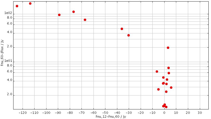
Click on 'Graphics' -> 'Plot' in the main TOPCAT window and plot Fnu_12 - Fnu_60 versus log(Fnu_60 - Jflux). This diagram is an adaptation of figure 5 of Acke and van den Ancker (2004, A&A, 426, 151). The shape of the mid-IR SED of a group I source is 'double-peaked' compared to the SED of a group II member. The x axis, IRAS Fnu_12 - Fnu_60, provides a quantitative measure for this difference in SED shape, whilst the y axis provides a measure for the differences in flux in the mid- and near-IR.
Where do we expect to see Group I and Group II objects in this plot?
Now lets take a look at the SEDs of some of these stars.
Open VOSPEC, either through the webstart or by running the .jar file.
Type 'HD 141569' in the Target field, '0.05' in the Size field and click 'Query'. HD 141569 corresponds to the source in column recno = 67 (i.e row 67 of the The catalogue table 2; IRAS 15473-0346).
The Server Selector window opens. The Spectra, Photometry and Theoretical Services available in the VO are listed in the left-hand region of the window. Click on each branch to open up the lists. Query all the spectral and photometric services by ticking the box 'Select all Observational' (located in the bottom left of the window). Click 'Query'.
The spectra are then loaded into the 'Spectra List' region of the main VOSpec window. This can be viewed also as a table by clicking the 'Tree/Table view' icon on the top right of the main VOSpec window.
Select spectra to view from various services, for example ISO, IUE/INES, ESO and FUSE. Check that you are loading spectra for the corr ect object by looking at (right-click on one spectra, and choose Properties), for example, Metadata fields: Target.Name, Distance... Click 'Retrieve' to get the data.
The spectra you've chosen are loaded into the main VOSpec window. To compare the SED with those in the above figure, change the y axis from Jy to erg/cm2/s by clicking on the 'Flux Unit' field to the left of the main VOSpec window.
Photometry can also be loaded into the SED from the CDS Multicatalogue Photometry Service. Change the view to Tree by clicking the 'Tree/Table view' icon . Tick the box to the left of the CDS Multicatalogue Photometry Service and all photometric points are selected. Click 'Retrieve'.
Each tree branch can be reorganised by the available metadata. Left click on the CDS Multicatalogue Photometry Service, select 'reorganize tree' and choose 'Catalogue' for the Level 1 criterion, and 'Distance (degrees)' for the Level 2 criterion, and click 'Organize'. The tree is now reorganised by catalogue and distance.
Which group would you initially classify the SED of HD 141569 into? Where does HD 141569 (column recno=67) fall in the TOPCAT plot Fnu_12 - Fnu_60 versus log(Fnu_60 - Jflux)?
Lets now pick a strong Group I candidate in the TOPCAT plot: the top left point. By clicking on the point in the scatter plot, the corresponding row is highlighted in the table.
This object is MWC 1080. Open another VOSpec and type MWC 1080 into the Target field, size '0.05' and click 'Query'.
Again tick the 'Select all Observational' box and click 'Query'.
Select spectra to view from various services, for example IUE/INES and ISO, and select photometry from the CDS Multicatalogue Photometry Service.
Change the y axis from Jy to erg/cm2/s.
Does the SED of MWC 1080 look like a Group I SED?
Additional:
Fitting lines:
Zoom into a region with a strong spectroscopic line.
Select Operations -> Fitting Utilities. The Fitting Window then opens. Select the Gaussian tab and click 'Generate'. The fitted Gaussian is plotted over the spectrum and the parameters used in the calculation are shown in the Fitting Window (where A=amplitude, x0 = central peak, sigma = standard deviation).
Finding Equivalent Widths:
Zoom into a region with a strong spectroscopic line.
Calculate the equivalent width of this line by selecting Operations -> Equivalent Width. The Analysis Window then opens. Click 'Calculate'. The equivalent width value appears in the 'Equivalent width value' field.
Perform a Kurucz model best fit to HD 141569 (an A0V star):
View just the FUSE and IUE spectra.
Select Operations -> Fitting Utilities. The Fitting Window then opens. In the TSAP Best Fit tab select the Kurucz ODFNEW/NOVER models and click 'Initiate'. A second window opens where you can choose an initial guess for the parameters, the closer to the best fit the shorter the computation time. Select teff =9500, log g = 4.00 and meta = 0.00 and click 'Start'.
When the best fit has been computed another window appears, be patient as this may take some time. Click 'LOAD'. The best fit Kurucz model is plotted along with the spectrum used to compute the best fit.
STILTS (Advanced Scripting with TOPCAT). We use STILTS to create a script. Below is a STILTS example that repeats the tutorial from points 1 to 22.
In TOPCAT, save table 2 that you downloaded in point 5 (called J_A+AS_104_315_table1), save it as Table2.xml
Run the following commands in the same directory as the stilts.jar. Alternatively, you can create a shell script and run this. See the STILTS help for help and more examples:
Zoom into a region with a strong spectroscopic line.
Select the Simple Line Access (Operations -> SLAP).
Highlight the region across the emission line. The selected region appears yellow and the Slap Viewer window opens. Within this window open the SLAP Services tree and select the different SLAP services. Then click 'select'.
A table appears for each service within the Slap Services Output field.
Go back to the main VOSpec window. By moving the cursor across the yellow region each atomic line that lies closest to the cursor is displayed. One can then identify the most likely atomic or molecular line.